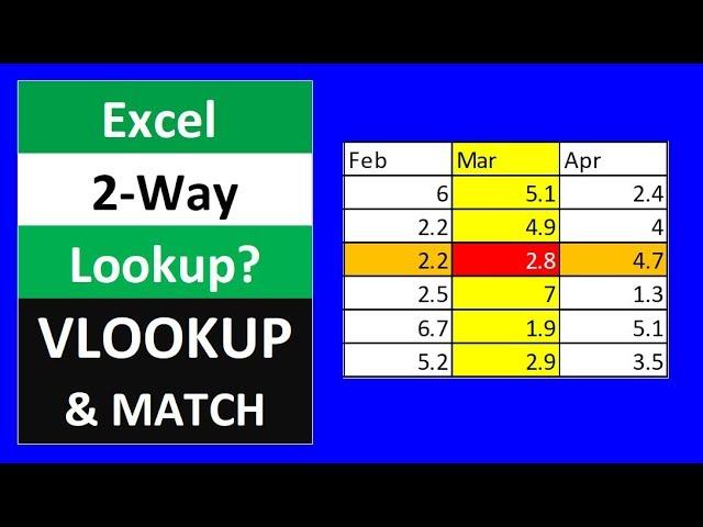
Excel Two Way Lookup with VLOOKUP & MATCH Functions - Excel Magic Trick 1567

Awesome..thanks!

Exactly what I needed, thank you so much! Been using excel for years and never knew about Match().

Many thanks. Very useful video!!

Excellent

Hi sir,
Hmare pass employee ka data h jisme jisme unki do I'd di gayi h, ek Regd I'd or dusri Employee I'd
Kya hm vlookup formula ka use karte hue dono I'd m se search karna chahte ya fr do me se kisi ek I'd se data search kr skte

Thank you so much sir

Superbly defined. Thanks

how to cosolidate all worksheet into one worksheet then sum up everythings?

it is possiable run by vba?

Hi Mike.. just for fun.. exercising my brain to think about other function combinations that would perform a 2-way lookup. Came up with these against your data set:
=OFFSET(C7,MATCH(B14,B7:B12,0)-1,MATCH(B15,C6:N6,0)-1)
=INDEX(C7:N12,MATCH(B14,B7:B12,0),MATCH(B15,C6:N6,0))
={SUM(IF(B7:B12=B14,IF(C6:N6=B15,C7:N12)))} - requires CSE
=HLOOKUP(B15,B6:N12,MATCH(B14,B6:B12,0),0)
The fun is endless at ExcelIsFun : )) Thumbs up!!

great and useful video sir. further can we extract values by vlookup from a cell or an array, having already a vlookup formula?

Thank you Mike. Hey Mike are you ever going to write another book? Slaying Excel Dragons was a blast and CTRL+Shift+Enter is a masterpiece. Just wondering if you had any plans to put something else out there in hardcopy.

Lovely video. Thanks for the share Mike.

Hi Mike, thanks for sharing. I just have a silly question as i just watched another video of yours about two way lookup using Index &Match. so what is the main differences of this method and Vlookup&Match for this two way lookup? Thanks a lot ~~

Nice and easy, great tip!

Btw, I've noticed that you count the column number for vlookup on this and some other videos. A small tip from me (although surely you're aware, but someone from the audience might not be) - if you start from the leftmost column of the lookup array and go right (with shift and right arrow key), there will be a tooltip near the cursor with the column count thus far, so when one reaches the desired column, they can make a mental note of it and keep extending the array (if needed). I find it really useful when number of columns is high.

a good one sir.

The dynamic conditional formatting is equally impressive as the combined lookup :-)

Thanks Mike.

How explaining the conditional formatting to highlight the row and column in yellow and the exact cell in red. I have a decent idea how to go about it, but wonder if you used a simpler method.

GREAT!

Grate that type of small vedio

Nice
👍

interesting

I use this all the time, it is a life saver, especially when the spreadsheet is owned by a 3rd party and they insist on adding and removing columns

Thumbs up!!!

This is not a example of two way lookup.

Very useful video Mike I personally love this combo VLOOKUP and MATCH, as MATCH makes the lookup array dynamic. Another approach can be adding a helper row in between rows 6 & 7 with numbers 1,2,3,4,5,6,7 so on in B7 to N7 cells, and then column index number will be delivered by HLOOKUP to assist VLOOKUP. But MATCH does is effortlessly. These videos are certainly adding new ides to our brains. Cheers :)

I love the combination of the two lookup functions, thanks Mike

Thanks Mike

Hi, Good Morning
I am an Indian and I am huge fan of you. Your video is very helpful for every Accountant so thank's a lot.

BEAUTIFUL!!!

Valuable because many users do not seem to be aware that VL can be used for efficient 2-way.

Hello dear, what is the use of this formula if I can just do it with one way? Like =vlookup(B14,B6:N12,5,0)

Thanks mike. Beautiful staff!!

Thanks for the revision :-)